Attenuation and OTDR Event Dead Zones Explained - OptiFiber Pro
Introduction
Testing multimode fiber cabling in high density environments requires a specialized OTDR capable of testing closely spaced connectors. Frequently, these connectors have high insertion loss and high reflectance. As a result, testing with an OTDR becomes difficult for all but the OTDRs with the highest spatial resolution.
At the heart of this type of OTDR are two components, a pulsed laser and avalanche photodiode (APD). The design of the electronics and more importantly, the type of APD selected, determines the deadzone performance.
All OTDR suppliers provide a deadzone specification. However, there are several things to consider when reviewing deadzones. First, the conditions under which the deadzone is specified must be considered. Second, how the deadzone changes as reflectance increases is important – something suppliers don’t specify. And third, what can one expect with deadzone performance in a real world fiber network.
Deadzone Specifications
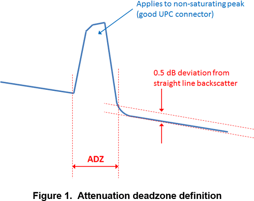
As shown in Figure 1, the attenuation deadzone (ADZ) is defined as the distance, usually for a single “good” connector reflective event, between the rising edge of the pulse to the 0.5 dB deviation from a straight line fit to the backscatter level. The backscatter level is the sloping line on the trace that provides the fiber attenuation value. This deadzone specification is usually given under best case conditions such as the shortest pulse width and best case connector reflectance.
The purpose of the ADZ specification is to provide an indication of the distance after a connector at which an accurate loss measurement can be made. From this definition, there might be an expectation that a patch cord, the length of the deadzone, can be concatenated to a previous connector to make a loss measurement. In reality, this may not be true.
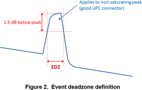
In Figure 2, the event deadzone (EDZ) is defined as the distance, usually for a single “good” connector, between two cursors set 1.5 dB below a reflective peak. This represents the full width half maximum pulse width in the linear domain. Again, this deadzone specification is usually given under best case conditions using the shortest pulse width and best case connector reflectance.
The purpose of the EDZ specification is to provide an indication of the distance after a connector at which an accurate length measurement can be made. From this definition there might be an expectation that a patch cord, the length of the deadzone, can be concatenated to a previous connector to make a length measurement. This is usually only true if both connectors both meet the criteria for the conditions under which the EDZ is specified (i.e. -45 dB reflectance). When the reflectance changes for either connector, the definition is no longer valid and the deadzone increases.
For both types of deadzones, the measurement is usually made at a single high quality connector. For the singlemode case, this might be made with a connector having a -52 dB reflectance. In the figures above, “non-saturating” implies a low connector reflectance, one that does not cause saturation and distortion in the OTDR receiver. When reflectance is high, deadzones increased due to a phenomenon intrinsic to APD’s called “tailing”.
Practical Deadzone Applications
Customer expectations for OTDR performance may be misaligned with OTDR specifications. Specifications are given with certain conditions usually described clearly in the footnotes.
For OTDRs, one should expect deadzone specifications to be limited to near end measurements under stated conditions. Deadzones should not be expected to remain constant with measurement length. Deadzones are a function of emitted pulses of finite width that become wider as measurement length increases (wide pulses are used for longer length measurements). Deadzones increase with reflectance in all but a few cases discussed later. Deadzone specifications are provided so a user might compare OTDR performance. However, the deadzone spec is defined for a single event, not as a network test.
More sophisticated OTDRs not only display a trace and event table, they also provide a graphical “map” of the fiber cabling under test. Mapping was first introduced in Premises-based OTDRs but has now become popular by many suppliers. The mapping information is derived from the same analysis used to generate an event table but is shown as a more easy to use schematic. Analyzer software is pushed to its limits when closely spaced connectors are to be measured, especially if each have different reflectances (i.e. clean connector followed by a scratched connector).
An example of an event deadzone expectation might be as follows. The event deadzone is specified as 1 meter. The fiber network has a 1 meter patch cord in the middle of two longer lengths. The user expects the OTDR to locate and identify the 1 meter patch cord and possibly make loss and reflectance measurements. The OTDR will be able to measure the length of the 1 meter patch cord only if the conditions of the specification have been satisfied; both reflectances must be within the restricted limits as defined within the specification footnote. Keep in mind that event deadzones only locate the reflectance peaks, so loss measurements are not possible.
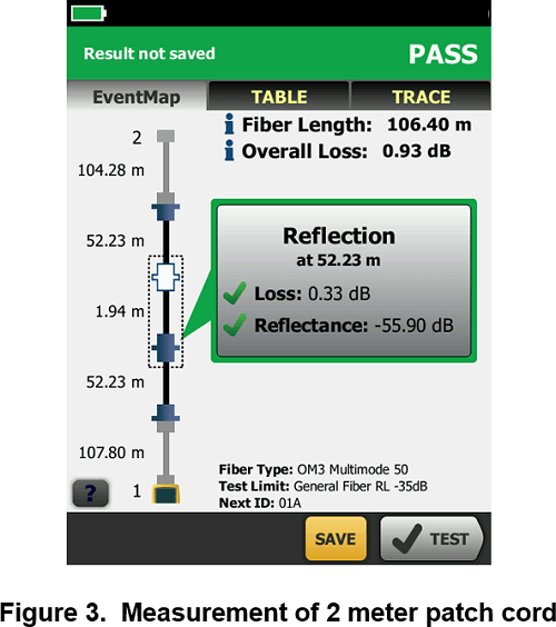
In another example, the attenuation deadzone claim is 2 meters. The fiber network has a 2 meter patch cord in the middle of two long lengths. The user expects to be able to measure the loss of the patch cord. If there is sufficient backscatter after each reflection as shown, the OTDR will be able to make the measurement.
In Figure 3, the first connector of the 1.94 meter length is identified with location, loss, and reflectance. Since two connectors are spaced close together, there may be limited backscatter after the first pulse. The second pulse may merge into the backscatter of the first pulse. As a result, the loss is measured from the backscatter of the second pulse to the end of backscatter at the front of the first pulse. Therefore, what is actually being measured is the loss of two pulses.
In Figure 4, the second pulse on the far side of the 1.94 meter patch cord cannot be identified and is labeled as a hidden event. This is because the start of the second pulse is being hidden within the backscatter of the first pulse. Therefore, this event cannot be measured fully.

Figure 5 shows that with enough distance between pulses, connector attenuation at both reflectances can easily be measured. Under these conditions, the attenuation deadzone per the OTDR specification can be verified.
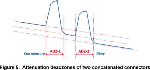
On the other hand, if the fiber network has a 2 meter patch cord in the middle of two long fibers, it might be difficult to make a reliable measurement since there is not enough backscatter after the first connector (reflectance) to make a straight line approximation.
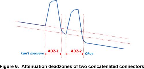
Figure 6 shows an example of two connectors place close together that might very well be the length of the attenuation deadzone specification. A skilled OTDR user might be able to make a manual measurement of the attenuation deadzones of both pulses. The analysis software, on the other hand, might measure the loss of the first connector (pulse) by taking the difference in backscatter from the start of the first pulse to the end of the second pulse.
Photodiodes
Frequently, OTDR designs will share one photodetector between two wavelengths. InGaAs detectors are commonly used in OTDRs to detect 1310 nm and 1550 nm for single-mode testing. For multimode testing there are two common options. The first is to use an InGaAs photodiode for both 850 nm and 1300 nm. InGaAs responds well to 1300 nm but has lower and frequently unspecified (by the APD supplier) responsivity at 850 nm. The second choice is to use two photodiodes, one InGaAs for 1300 nm multimode and one to Si (Silicon) for 850 nm multimode.
Not only does Si respond well at 850 nm, it also has much higher internal gain (a characteristic of APDs) than an InGaAs device. The photodiodes used for OTDRs have internal gain called the multiplication factor. This internal gain greatly improves the signal to noise ratio which is related to instrument dynamic range. As an example, an InGaAs APD might have a multiplication factor of 30 while the Si APD might have a multiplication factor of 70. This means for a given backscatter level, a more narrow pulse can be used which improves spatial resolution.
Deadzone vs. Reflectance for InGaAs and Si
As mentioned earlier, the deadzone typically increases as reflectance increases, and is especially troublesome when using InGaAs photodetectors. Si is much better.
The following two graphs are composed from data taken from two OTDRs using either a Si APD or an InGaAs APD. The InGaAs data, although taken at 1550 nm, would have the same type of deadzone response at any wavelength including 850 nm. Similar pulse widths were used for 850 nm and 1310 nm.
The data below shows the relationship between deadzones and connector reflectance at 1550 nm using an InGaAs photodiode commonly used in OTDRs. The first graph in Figure 7 shows the 850 nm event deadzone (EDZ) and attenuation deadzone (ADZ) as the reflectance increases from a value for a typical UPC connector (-45 dB) to a connector with high reflectance (i.e. dirty connector).
The data shows that the EDZ is not affected by reflectance. This is because the measurement is made below a non-saturated peak. If the peak became saturated (i.e. “flat top”), the EDZ would increase but this is related to the design of the OTDR. For the ADZ, there is a gradual increase from 2 meters to 2.75 meters but at -26 dB reflectance, there is deflection and the ADZ increases to 4.5 meters when reflectance is -25 dB. Despite the increase in ADZ over this range, it is much better than what the ADZ might be using an InGaAs APD as shown in Figure 8.
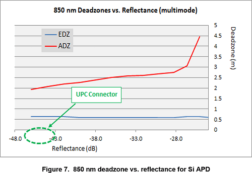
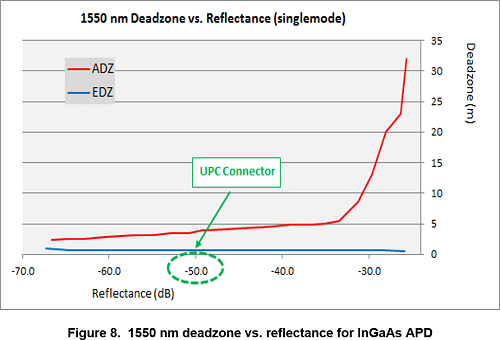
Figure 8 shows the 1550 nm deadzone performance for an InGaAs APD as reflectance is increased. This graph shows the EDZ and ADZ as the reflectance increases from a typical UPC connector at -51 dB to a connector with high reflectance at -30 dB (i.e. dirty connector). The EDZ is not affected by reflectance but the ADZ slowly increases from 4.5 meters to 5 meters over a 15 dB range then quickly increases at -30 dB and reaches over 30 meters of ADZ. The ADZ will continue to increase as reflectance increases. Unless complicated provision is made for single-mode OTDRs, they all suffer from this phenomenon when an InGaAs APD is used.
Summary
Si APDs offer superior performance when testing multimode fiber at 850 nm when compared to InGaAs APDs used with OTDRs. Si APDs have better signal to noise ratios which encourages use of narrow pulse interrogation and analysis of installed fiber cabling. Si APDs suffer much less tailing when subjected to optical overload caused by high reflectance at connectors. High reflectance is arguably the most common problem found by OTDRs during fiber network testing. The data has shown that OTDRs employing Si APDs have performance advantages over other types of OTDRs, especially in high resolution applications.
While there might be a premium for high performance OTDRs, for the user comparing specifications from OTDR suppliers, it is not evident if a Si APD is used unless an evaluation under high reflectance is made.
All Videos in This Series

Related Products
CertiFiber® Pro Optical Loss Test Set
OptiFiber® Pro OTDR Family

Fiber Optic Cleaning Kits